Linear Regression in RDr. D’Agostino McGowan1 / 37

Let's look at an example

Let's look at a sample of 116 sparrows from Kent Island. We are interested in the relationship between Weight and Wing Length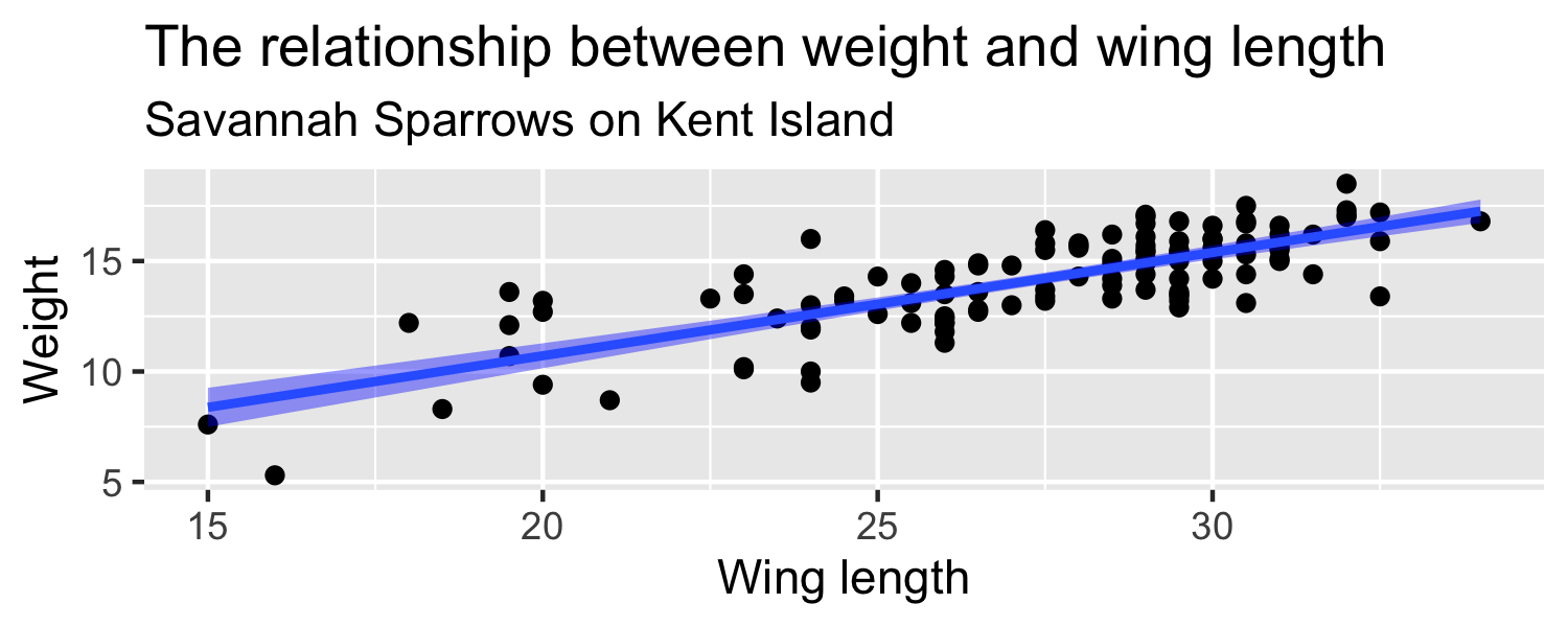

the standard error of $\hat{\beta_1}$ ( $SE_{\hat{\beta}_1}$ ) is how much we expect the sample slope to vary from one random sample to another.

2 / 37

Sparrows

How can we quantify how much we'd expect the slope to differ from one random sample to another?

linear_reg() %>%
  set_engine("lm") %>%
  fit(Weight ~ WingLength, data = Sparrows) %>%
  tidy()

## # A tibble: 2 x 5
##   term        estimate std.error statistic  p.value
##   <chr>          <dbl>     <dbl>     <dbl>    <dbl>
## 1 (Intercept)    1.37     0.957       1.43 1.56e- 1
## 2 WingLength     0.467    0.0347     13.5  2.62e-25

3 / 37

Sparrows

How do we interpret this?

linear_reg() %>%
  set_engine("lm") %>%
  fit(Weight ~ WingLength, data = Sparrows) %>%
  tidy()

## # A tibble: 2 x 5
##   term        estimate std.error statistic  p.value
##   <chr>          <dbl>     <dbl>     <dbl>    <dbl>
## 1 (Intercept)    1.37     0.957       1.43 1.56e- 1
## 2 WingLength     0.467    0.0347     13.5  2.62e-25

4 / 37

Sparrows

How do we interpret this?

linear_reg() %>%
  set_engine("lm") %>%
  fit(Weight ~ WingLength, data = Sparrows) %>%
  tidy()

## # A tibble: 2 x 5
##   term        estimate std.error statistic  p.value
##   <chr>          <dbl>     <dbl>     <dbl>    <dbl>
## 1 (Intercept)    1.37     0.957       1.43 1.56e- 1
## 2 WingLength     0.467    0.0347     13.5  2.62e-25

"the sample slope is more than 13 standard errors above a slope of zero"

5 / 37

Sparrows

How do we know what values of this statistic are worth paying attention to?

linear_reg() %>%
  set_engine("lm") %>%
  fit(Weight ~ WingLength, data = Sparrows) %>%
  tidy()

## # A tibble: 2 x 5
##   term        estimate std.error statistic  p.value
##   <chr>          <dbl>     <dbl>     <dbl>    <dbl>
## 1 (Intercept)    1.37     0.957       1.43 1.56e- 1
## 2 WingLength     0.467    0.0347     13.5  2.62e-25

6 / 37

Sparrows

How do we know what values of this statistic are worth paying attention to?

linear_reg() %>%
  set_engine("lm") %>%
  fit(Weight ~ WingLength, data = Sparrows) %>%
  tidy()

## # A tibble: 2 x 5
##   term        estimate std.error statistic  p.value
##   <chr>          <dbl>     <dbl>     <dbl>    <dbl>
## 1 (Intercept)    1.37     0.957       1.43 1.56e- 1
## 2 WingLength     0.467    0.0347     13.5  2.62e-25

confidence intervals
p-values

7 / 37

Sparrows

How do we know what values of this statistic are worth paying attention to?

linear_reg() %>%
  set_engine("lm") %>%
  fit(Weight ~ WingLength, data = Sparrows) %>%
  tidy(conf.int = TRUE)

## # A tibble: 2 x 7
##   term        estimate std.error statistic  p.value conf.low conf.high
##   <chr>          <dbl>     <dbl>     <dbl>    <dbl>    <dbl>     <dbl>
## 1 (Intercept)    1.37     0.957       1.43 1.56e- 1   -0.531     3.26 
## 2 WingLength     0.467    0.0347     13.5  2.62e-25    0.399     0.536

confidence intervals
p-values

8 / 37

Dr. Lucy D'Agostino McGowan

 Application ExerciseFit a linear model using the mtcars data frame predicting miles per gallon (mpg) from (wt)
Pull out the coefficients and confidence intervals using the tidy() function demonstrated. How do you interpret these?

04:00
9 / 37

Sparrows

How are these statistics distributed under the null hypothesis?

linear_reg() %>%
  set_engine("lm") %>%
  fit(Weight ~ WingLength, data = Sparrows) %>%
  tidy()

## # A tibble: 2 x 5
##   term        estimate std.error statistic  p.value
##   <chr>          <dbl>     <dbl>     <dbl>    <dbl>
## 1 (Intercept)    1.37     0.957       1.43 1.56e- 1
## 2 WingLength     0.467    0.0347     13.5  2.62e-25

10 / 37

Spar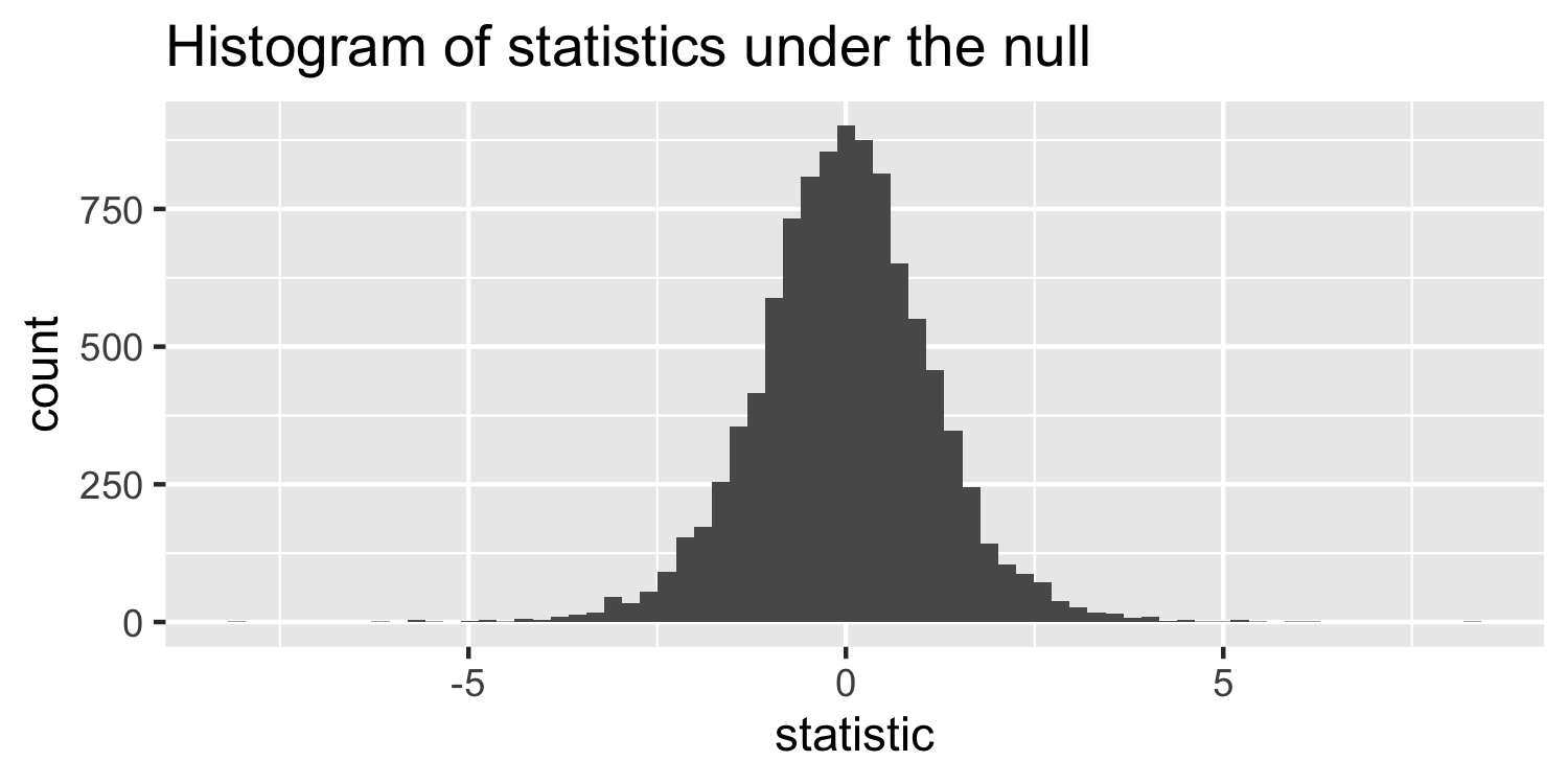rows

I've generated some data under a null hypothesis where $n = 20$

11 / 37

Spar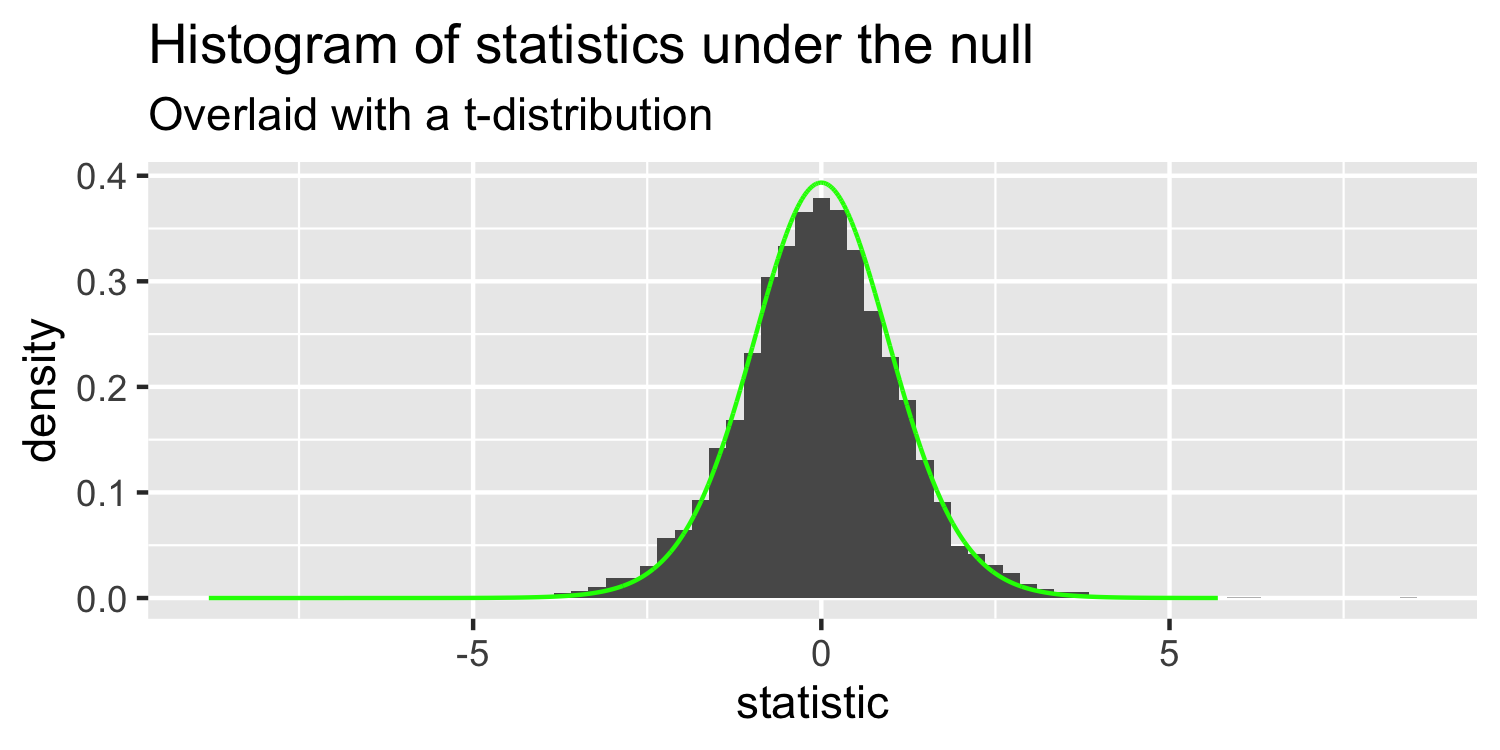rows

this is a t-distribution with n-p-1 degrees of freedom.

12 / 37

Sparrows

The distribution of test statistics we would expect given the null hypothesis is true, $\beta_1 = 0$, is t-distribution with n-2 degrees of freedom.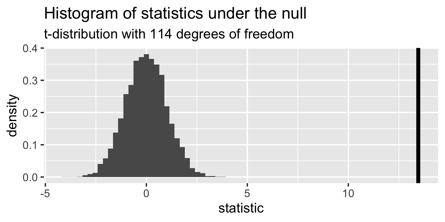

13 / 37

Sparrows

14 / 37

Sparrows

How can we compare this line to the distribution under the null?

15 / 37

Sparrows

How can we compare this line to the distribution under the null?

p-value

15 / 37

p-value

The probability of getting a statistic as extreme or more extreme than the observed test statistic given the null hypothesis is true

16 / 37

Sparrows

linear_reg() %>%
  set_engine("lm") %>%
  fit(Weight ~ WingLength, data = Sparrows) %>%
  tidy()

## # A tibble: 2 x 5
##   term        estimate std.error statistic  p.value
##   <chr>          <dbl>     <dbl>     <dbl>    <dbl>
## 1 (Intercept)    1.37     0.957       1.43 1.56e- 1
## 2 WingLength     0.467    0.0347     13.5  2.62e-25

17 / 37

Return to generated data, n = 20

Let's say we get a statistic of 1.5 in a sample

18 / 37

Let's do it in R!

The proportion of area less than 1.5

pt(1.5, df = 18)

## [1] 0.9245248

19 / 37

Let's do it in R!

The proportion of area greater than 1.5

pt(1.5, df = 18, lower.tail = FALSE)

## [1] 0.07547523

20 / 37

Let's do it in R!

The proportion of area greater than 1.5 or less than -1.5.

21 / 37

Let's do it in R!

The proportion of area greater than 1.5 or less than -1.5.

pt(1.5, df = 18, lower.tail = FALSE) * 2

## [1] 0.1509505

21 / 37

p-value

The probability of getting a statistic as extreme or more extreme than the observed test statistic given the null hypothesis is true

22 / 37

Dr. Lucy D'Agostino McGowan

Hypothesis testnull hypothesis \(H_0: \beta_1 = 0\) 
alternative hypothesis \(H_A: \beta_1 \ne 0\)
23 / 37

Dr. Lucy D'Agostino McGowan

Hypothesis testnull hypothesis \(H_0: \beta_1 = 0\) 
alternative hypothesis \(H_A: \beta_1 \ne 0\)
p-value: 0.15
23 / 37

Dr. Lucy D'Agostino McGowan

Hypothesis testnull hypothesis \(H_0: \beta_1 = 0\) 
alternative hypothesis \(H_A: \beta_1 \ne 0\)
p-value: 0.15
Often, we have an \(\alpha\)-level cutoff to compare this to, for example 0.05. Since this is greater than 0.05, we fail to reject the null hypothesis
23 / 37

`Application Exercise`

Using the linear model you fit previously (mpg from wt using the mtcars data) - calculate the p-value for the coefficient for weight? Interpret this value. What is the null hypothesis? What is the alternative hypothesis? Do you reject the null?

04:00

24 / 37

confidence intervals

If we use the same sampling method to select different samples and computed an interval estimate for each sample, we would expect the true population parameter ( $\beta_1$ ) to fall within the interval estimates 95% of the time.

25 / 37

Confidence interval

$\Huge \hat\beta_1 \pm t^∗ \times SE_{\hat\beta_1}$

26 / 37

Confidence interval

$\Huge \hat\beta_1 \pm t^∗ \times SE_{\hat\beta_1}$

$t^*$ is the critical value for the $t_{n−p-1}$ density curve to obtain the desired confidence level

27 / 37

Confidence interval

$\Huge \hat\beta_1 \pm t^∗ \times SE_{\hat\beta_1}$

$t^*$ is the critical value for the $t_{n−p-1}$ density curve to obtain the desired confidence level
Often we want a 95% confidence level.

27 / 37

Dr. Lucy D'Agostino McGowan

Let's do it in R!linear_reg() %>%
  set_engine("lm") %>%
  fit(Weight ~ WingLength, data = Sparrows) %>%
  tidy(conf.int = TRUE)

## # A tibble: 2 x 7
##   term        estimate std.error statistic  p.value conf.low conf.high
##   <chr>          <dbl>     <dbl>     <dbl>    <dbl>    <dbl>     <dbl>
## 1 (Intercept)    1.37     0.957       1.43 1.56e- 1   -0.531     3.26 
## 2 WingLength     0.467    0.0347     13.5  2.62e-25    0.399     0.536
\(t^* = t_{n-p-1} = t_{114} = 1.98\)
28 / 37

Dr. Lucy D'Agostino McGowan

Let's do it in R!linear_reg() %>%
  set_engine("lm") %>%
  fit(Weight ~ WingLength, data = Sparrows) %>%
  tidy(conf.int = TRUE)

## # A tibble: 2 x 7
##   term        estimate std.error statistic  p.value conf.low conf.high
##   <chr>          <dbl>     <dbl>     <dbl>    <dbl>    <dbl>     <dbl>
## 1 (Intercept)    1.37     0.957       1.43 1.56e- 1   -0.531     3.26 
## 2 WingLength     0.467    0.0347     13.5  2.62e-25    0.399     0.536
\(t^* = t_{n-p-1} = t_{114} = 1.98\)
\(LB = 0.47 - 1.98\times 0.0347 = 0.399\)
\(UB = 0.47+1.98 \times 0.0347 = 0.536\)
28 / 37

confidence intervals

29 / 37

Dr. Lucy D'Agostino McGowan

Linear Regression Questions✔️ Is there a relationship between a response variable and predictors? 
✔️ How strong is the relationship? 
✔️ What is the uncertainty? 
How accurately can we predict a future outcome?
30 / 37

Sparrows

Using the information here, how could I predict a new sparrow's weight if I knew the wing length was 30?

linear_reg() %>%
  set_engine("lm") %>%
  fit(Weight ~ WingLength, data = Sparrows) %>%
  tidy()

## # A tibble: 2 x 5
##   term        estimate std.error statistic  p.value
##   <chr>          <dbl>     <dbl>     <dbl>    <dbl>
## 1 (Intercept)    1.37     0.957       1.43 1.56e- 1
## 2 WingLength     0.467    0.0347     13.5  2.62e-25

31 / 37

Sparrows

Using the information here, how could I predict a new sparrow's weight if I knew the wing length was 30?

linear_reg() %>%
  set_engine("lm") %>%
  fit(Weight ~ WingLength, data = Sparrows) %>%
  tidy()

## # A tibble: 2 x 5
##   term        estimate std.error statistic  p.value
##   <chr>          <dbl>     <dbl>     <dbl>    <dbl>
## 1 (Intercept)    1.37     0.957       1.43 1.56e- 1
## 2 WingLength     0.467    0.0347     13.5  2.62e-25

$1.37 + 0.467 \times 30 = 15.38$

31 / 37

Linear Regression Accuracy

What is the residual sum of squares again?

Note: In previous classes, this may have been referred to as SSE (sum of squares error), the book uses RSS, so we will stick with that!

32 / 37

Linear Regression Accuracy

What is the residual sum of squares again?

Note: In previous classes, this may have been referred to as SSE (sum of squares error), the book uses RSS, so we will stick with that!

$$RSS = \sum(y_i - \hat{y}_i)^2$$

32 / 37

Linear Regression Accuracy

What is the residual sum of squares again?

Note: In previous classes, this may have been referred to as SSE (sum of squares error), the book uses RSS, so we will stick with that!

$$RSS = \sum(y_i - \hat{y}_i)^2$$

The total sum of squares represents the variability of the outcome, it is equivalent to the variability described by the model plus the remaining residual sum of squares

$$TSS = \sum(y_i - \bar{y})^2$$

32 / 37

Dr. Lucy D'Agostino McGowan

Linear Regression AccuracyThere are many ways "model fit" can be assessed. Two common ones are:Residual Standard Error (RSE)
\(R^2\) - the fraction of the variance explained

33 / 37

Dr. Lucy D'Agostino McGowan

Linear Regression AccuracyThere are many ways "model fit" can be assessed. Two common ones are:Residual Standard Error (RSE)
\(R^2\) - the fraction of the variance explained

\(RSE = \sqrt{\frac{1}{n-p-1}RSS}\)
33 / 37

Dr. Lucy D'Agostino McGowan

Linear Regression AccuracyThere are many ways "model fit" can be assessed. Two common ones are:Residual Standard Error (RSE)
\(R^2\) - the fraction of the variance explained

\(RSE = \sqrt{\frac{1}{n-p-1}RSS}\)
\(R^2 = 1 - \frac{RSS}{TSS}\)
33 / 37

Linear Regression Accuracy

What could we use to determine whether at least one predictor is useful?

34 / 37

Linear Regression Accuracy

What could we use to determine whether at least one predictor is useful?

$$F = \frac{(TSS - RSS)/p}{RSS/(n-p-1)}\sim F_{p,n-p-1}$$ We can use a F-statistic!

34 / 37

Dr. Lucy D'Agostino McGowan

Let's do it in R!lm_fit <- linear_reg() %>%
  set_engine("lm") %>%
  fit(Weight ~ WingLength, data = Sparrows)
glance(lm_fit$fit)

## # A tibble: 1 x 12
##   r.squared adj.r.squared sigma statistic  p.value    df logLik   AIC   BIC
##       <dbl>         <dbl> <dbl>     <dbl>    <dbl> <dbl>  <dbl> <dbl> <dbl>
## 1     0.614         0.611  1.40      181. 2.62e-25     1  -203.  411.  419.
## # … with 3 more variables: deviance <dbl>, df.residual <int>, nobs <int>
35 / 37

`Application Exercise`

Using the model previously fit (using the mtcars data predicting miles per gallon from weight), pull out the F-statistic and $R^2$ using the glance() function. Interpret these values.

04:00

36 / 37

Additional Linear Regression Topics

Polynomial terms
Interactions
Outliers
Non-constant variance of error terms
High leverage points
Collinearity

Refer to Chapter 3 for more details on these topics if you need a refresher.

37 / 37

Help

Keyboard shortcuts

↑, ←, Pg Up, k

Go to previous slide

↓, →, Pg Dn, Space, j

Go to next slide

Home

Go to first slide

End

Go to last slide

Number + Return

Go to specific slide

b / m / f

Toggle blackout / mirrored / fullscreen mode

Clone slideshow

Toggle presenter mode

Restart the presentation timer

?, h

Toggle this help