Logistic regression

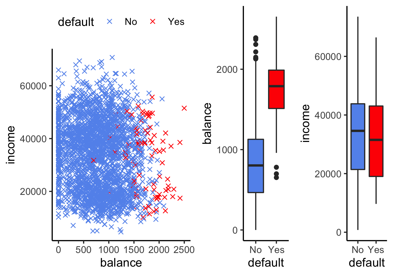
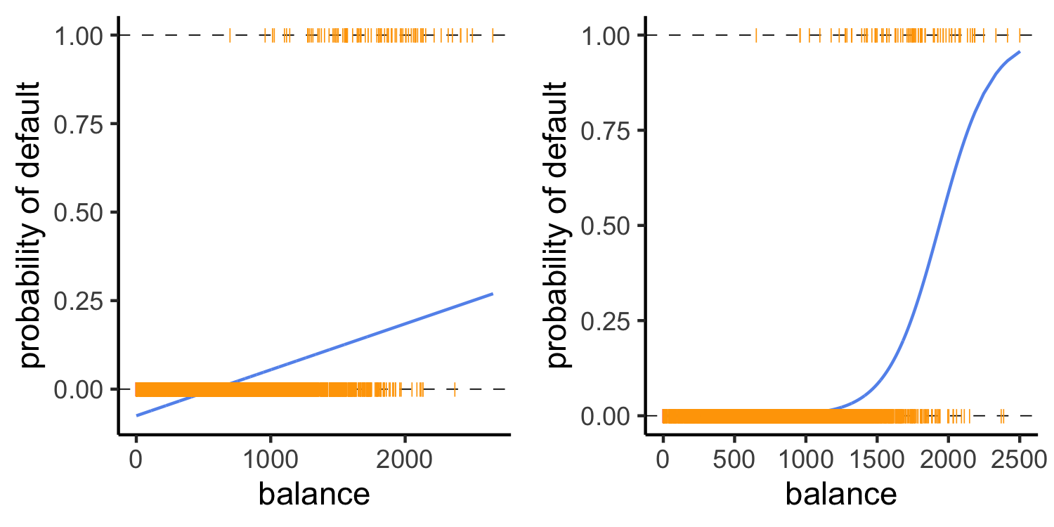
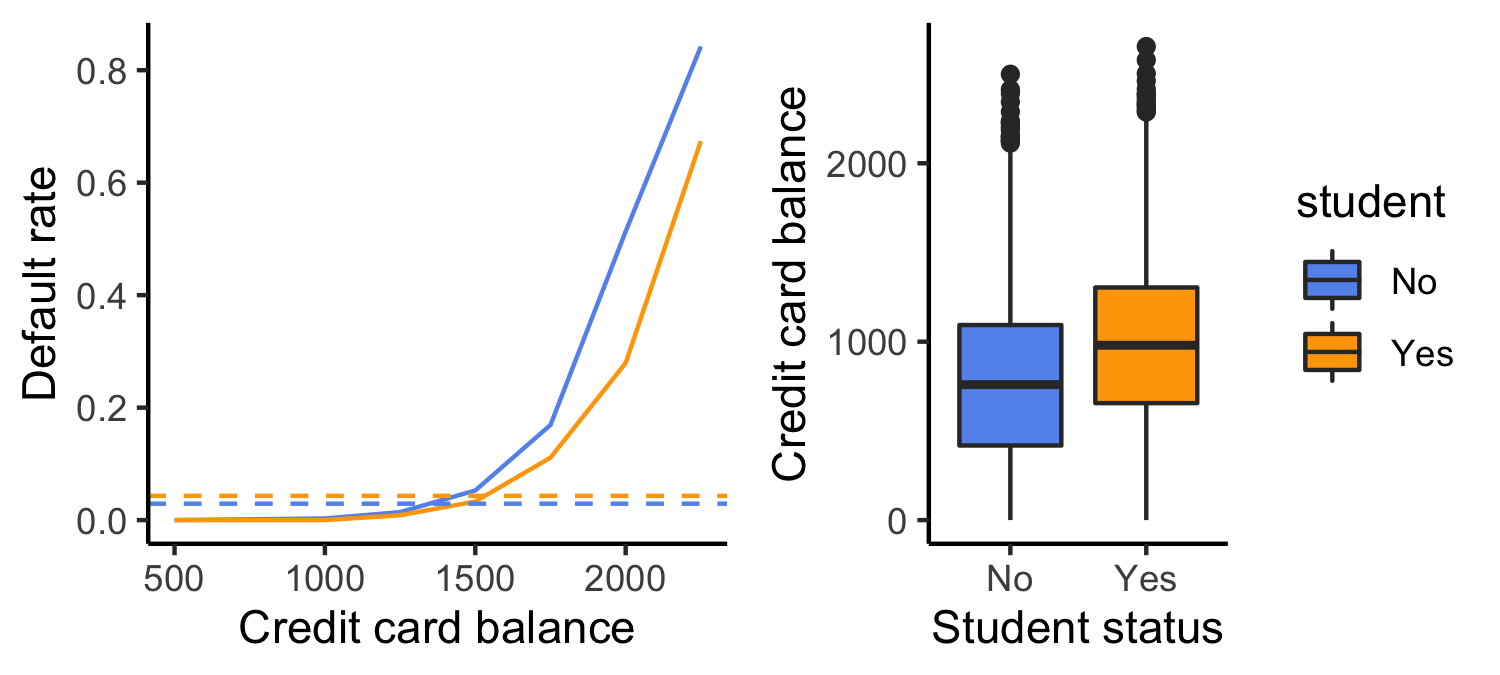
# Logistic regression
### Dr. D’Agostino McGowan

---

<div class="my-footer">
<span>
Dr. Lucy D'Agostino McGowan <i>adapted from slides by Hastie & Tibshirani</i>
</span>
</div>

---

## Recap

* Last class we had a _linear regression_ refresher
--

* We covered how to write a linear model in _matrix_ form
--

* We learned how to minimize RSS to calculate `$\hat{\beta}$` with `$(\mathbf{X^TX)^{-1}X^Ty}$`
--

* Linear regression is a great tool when we have a continuous outcome
* We are going to learn some fancy ways to do even better in the future
---

# Classification

---

## Classification

.question[
What are some examples of classification problems?
]
* Qualitative response variable in an _unordered set_, `$\mathcal{C}$`  
--

* `eye color` `$\in$` `{blue, brown, green}`
  * `email` `$\in$` `{spam, not spam}`
--

* Response, `$Y$` takes on values in `$\mathcal{C}$`
* Predictors are a vector, `$X$`
--

* The task: build a function `$C(X)$` that takes `$X$` and predicts `$Y$`, `$C(X)\in\mathcal{C}$` 
--

* Many times we are actually more interested in the _probabilities_ that `$X$` belongs to each category in `$\mathcal{C}$`

---

## Example: Credit card default

![](09-logistic_files/figure-html/plot1-1.png)

---

## Can we use linear regression?

We can code `Default` as

`$$Y = \begin{cases} 0 & \textrm{if }\texttt{No}\\ 1&\textrm{if }\texttt{Yes}\end{cases}$$`
Can we fit a linear regression of `$Y$` on `$X$` and classify as `Yes` if `$\hat{Y}> 0.5$`?

* In this case of a **binary** outcome, linear regression is okay (it is equivalent to **linear discriminant analysis**, you can read more about that in your book!)
* `$E[Y|X=x] = P(Y=1|X=x)$`, so it seems like this is a pretty good idea!
* **The problem**: Linear regression can produce probabilities less than 0 or greater than 1 😱
--
.question[
What may do a better job?
]
--

* **Logistic regression!**

---

## Linear versus logistic regression

![](09-logistic_files/figure-html/plot2-1.png)

* The orange marks represent the response `$Y\in\{0,1\}$`

---

## Linear Regression

What if we have `$>2$` possible outcomes? For example, someone comes to the emergency room and we need to classify them according to their symptoms

$$ 
`\begin{align}
Y = \begin{cases} 1& \textrm{if }\texttt{stroke}\\2&\textrm{if }\texttt{drug overdose}\\3&\textrm{if }\texttt{epileptic seizure}\end{cases}
\end{align}`
$$

* The coding implies an _ordering_
* The coding implies _equal spacing_ (that is the difference between `stroke` and `drug overdose` is the same as `drug overdose` and `epileptic seizure`)
---

## Linear Regression

What if we have `$>2$` possible outcomes? For example, someone comes to the emergency room and we need to classify them according to their symptoms

$$ 
`\begin{align}
Y = \begin{cases} 1& \textrm{if }\texttt{stroke}\\2&\textrm{if }\texttt{drug overdose}\\3&\textrm{if }\texttt{epileptic seizure}\end{cases}
\end{align}`
$$

* Linear regression is **not** appropriate here
* **Mutliclass logistic regression** or **discriminant analysis** are more appropriate

---

## Logistic Regression

$$ 
p(X) = \frac{e^{\beta_0+\beta_1X}}{1+e^{\beta_0+\beta_1X}}
$$

* Note: `$p(X)$` is shorthand for `$P(Y=1|X)$`
* No matter what values `$\beta_0$`, `$\beta_1$`, or `$X$` take `$p(X)$` will always be between 0 and 1
--

* We can rearrange this into the following form:
$$
\log\left(\frac{p(X)}{1-p(X)}\right) = \beta_0 + \beta_1 X
$$

* This is a **log odds** or **logit** transformation of `$p(X)$`

---

## Linear versus logistic regression

![](09-logistic_files/figure-html/unnamed-chunk-3-1.png)

Logistic regression ensures that our estimates for `$p(X)$` are between 0 and 1 🎉

---

## Maximum Likelihood

]

---

## Maximum Likelihood

]

In logistic regression, we use **maximum likelihood** to estimate the parameters

`$$\mathcal{l}(\beta_0,\beta_1)=\prod_{i:y_i=1}p(x_i)\prod_{i:y_i=0}(1-p(x_i))$$`
--

* This **likelihood** give the probability of the observed ones and zeros in the data
* We pick `$\beta_0$` and `$\beta_1$` to maximize the likelihood
* _We'll let `R` do the heavy lifting here_

---

## Let's see it in R

```r
logistic_reg() %>%
  set_engine("glm") %>%
  fit(default ~ balance, 
      data = Default) %>%
  tidy()
```

```
## # A tibble: 2 x 5
##   term         estimate std.error statistic   p.value
##   <chr>           <dbl>     <dbl>     <dbl>     <dbl>
## 1 (Intercept) -10.7      0.361        -29.5 3.62e-191
## 2 balance       0.00550  0.000220      25.0 1.98e-137
```
]

* Use the `logistic_reg()` function in R with the `glm` engine

---

## Making predictions

$$
\hat{p}(X) = \frac{e^{\hat{\beta}_0+\hat{\beta}_1X}}{1+e^{\hat{\beta}_0+\hat{\beta}_1X}}=\frac{e^{-10.65+0.0055\times 1000}}{1+e^{-10.65+0.0055\times 1000}}=0.006
$$

---

## Making predictions

$$
\hat{p}(X) = \frac{e^{\hat{\beta}_0+\hat{\beta}_1X}}{1+e^{\hat{\beta}_0+\hat{\beta}_1X}}=\frac{e^{-10.65+0.0055\times 2000}}{1+e^{-10.65+0.0055\times 2000}}=0.586
$$

---

## Logistic regression example

Let's refit the model to predict the probability of default given the customer is a `student`

`$$P(\texttt{default = Yes}|\texttt{student = Yes}) = \frac{e^{-3.5041+0.4049\times1}}{1+e^{-3.5041+0.4049\times1}}=0.0431$$`
--

`$$P(\texttt{default = Yes}|\texttt{student = No}) = \frac{e^{-3.5041+0.4049\times0}}{1+e^{-3.5041+0.4049\times0}}=0.0292$$`

---

## Multiple logistic regression

`$$\log\left(\frac{p(X)}{1-p(X)}\right)=\beta_0+\beta_1X_1+\dots+\beta_pX_p$$`
`$$p(X) = \frac{e^{\beta_0+\beta_1X_1+\dots+\beta_pX_p}}{1+e^{\beta_0+\beta_1X_1+\dots+\beta_pX_p}}$$`

<table>
 <thead>
  <tr>
   <th style="text-align:left;"> term </th>
   <th style="text-align:right;"> estimate </th>
   <th style="text-align:right;"> std.error </th>
   <th style="text-align:right;"> statistic </th>
   <th style="text-align:right;"> p.value </th>
  </tr>
 </thead>
<tbody>
  <tr>
   <td style="text-align:left;"> (Intercept) </td>
   <td style="text-align:right;"> -10.8690452 </td>
   <td style="text-align:right;"> 0.4922555 </td>
   <td style="text-align:right;"> -22.080088 </td>
   <td style="text-align:right;"> 0.0000000 </td>
  </tr>
  <tr>
   <td style="text-align:left;"> balance </td>
   <td style="text-align:right;"> 0.0057365 </td>
   <td style="text-align:right;"> 0.0002319 </td>
   <td style="text-align:right;"> 24.737563 </td>
   <td style="text-align:right;"> 0.0000000 </td>
  </tr>
  <tr>
   <td style="text-align:left;"> income </td>
   <td style="text-align:right;"> 0.0000030 </td>
   <td style="text-align:right;"> 0.0000082 </td>
   <td style="text-align:right;"> 0.369815 </td>
   <td style="text-align:right;"> 0.7115203 </td>
  </tr>
  <tr>
   <td style="text-align:left;"> studentYes </td>
   <td style="text-align:right;"> -0.6467758 </td>
   <td style="text-align:right;"> 0.2362525 </td>
   <td style="text-align:right;"> -2.737646 </td>
   <td style="text-align:right;"> 0.0061881 </td>
  </tr>
</tbody>
</table>

--
* Why is the coefficient for `student` negative now when it was positive before?

---

## Confounding

![](09-logistic_files/figure-html/plot3-1.png)

## Confounding

![](09-logistic_files/figure-html/unnamed-chunk-9-1.png)

* Students tend to have higher balances than non-students
  * Their **marginal** default rate is higher
--

* For each level of balance, students default less 
  * Their **conditional** default rate is lower

---

## Logistic regression for more than two classes

* So far we've discussed **binary** outcome data
* We can generalize this to situations with **multiple** classes

`$$P(Y=k|X) = \frac{e ^{\beta_{0k}+\beta_{1k}X_1+\dots+\beta_{pk}X_p}}{\sum_{l=1}^Ke^{\beta_{0l}+\beta_{1l}X_1+\dots+\beta_{pl}X_p}}$$`

* Here we have a linear function for **each** of the `$K$` classes
* This is known as **multinomial logistic regression**

---