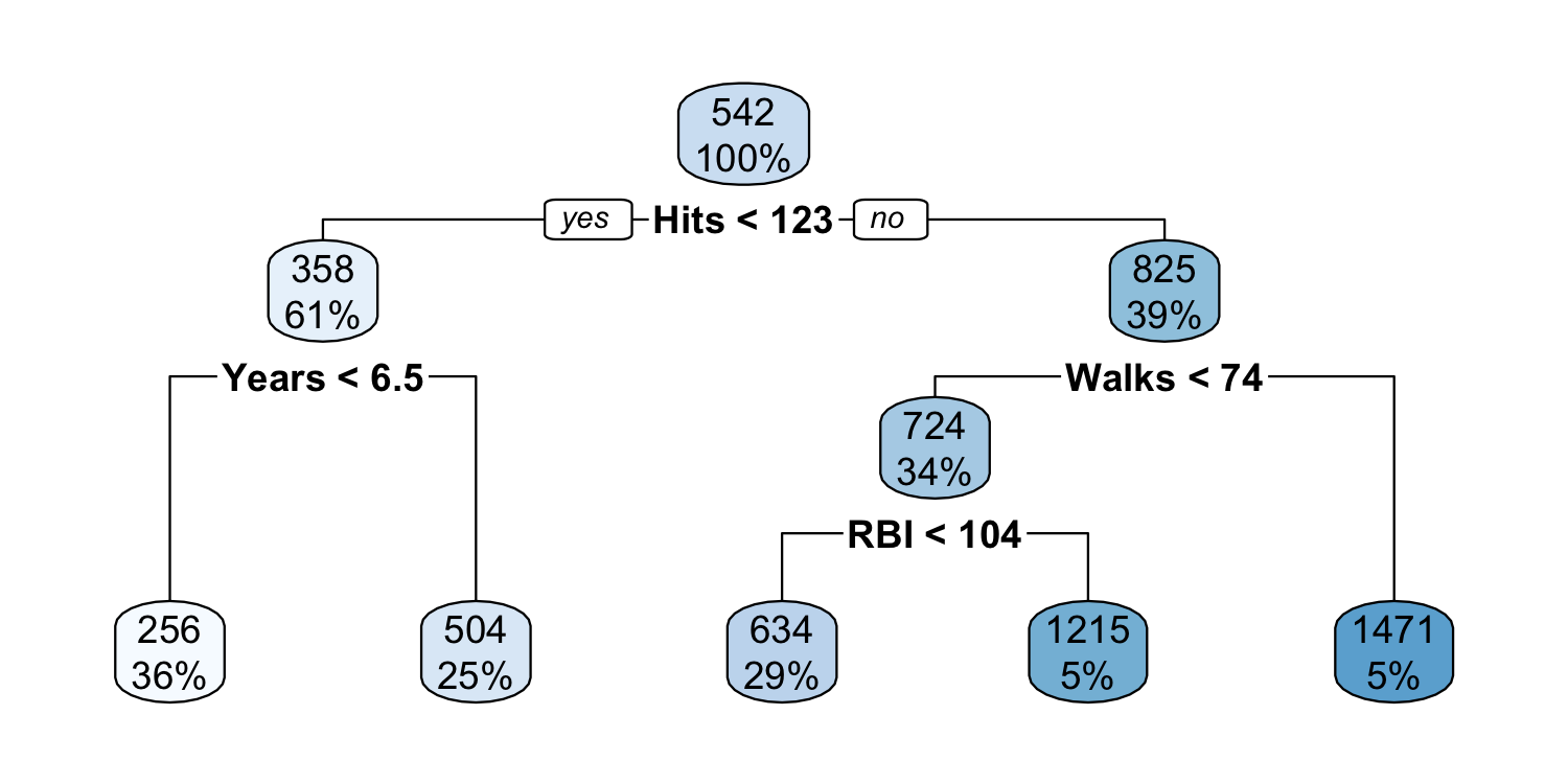
class: center, middle, inverse, title-slide # Decision trees - Regression tree example ### Dr. D’Agostino McGowan --- layout: true <div class="my-footer"> <span> Dr. Lucy D'Agostino McGowan <i>adapted from slides by Hastie & Tibshirani</i> </span> </div> --- class: center, middle ## The baseball example --- ## 1. Randomly divide the data in half, 132 training observations, 131 testing ```r set.seed(77) baseball_split <- initial_split(baseball, prop = 0.5) baseball_train <- training(baseball_split) ``` --- ## 2. Create cross-validation object for 6-fold cross validation ```r baseball_cv <- vfold_cv(baseball_train, v = 6) ``` --- ## 3. Create a model specification that tunes based on complexity, `\(\alpha\)` ```r tree_spec <- decision_tree( cost_complexity = tune(), tree_depth = 10, mode = "regression") %>% set_engine("rpart") ``` -- .question[ What is my tree depth for my "large" tree? ] --- ## 4. Fit the model on the cross validation set .small[ ```r grid <- expand_grid(cost_complexity = seq(0.01, 0.05, by = 0.01)) model <- tune_grid(tree_spec, Salary ~ Hits + Years + PutOuts + RBI + Walks + Runs, grid = grid, resamples = baseball_cv) ``` ] -- .question[ What `\(\alpha\)`s am I trying? ] --- ## 5. Choose `\(\alpha\)` that minimizes the RMSE ```r model %>% collect_metrics() %>% filter(.metric == "rmse") %>% arrange(mean) ``` ``` ## # A tibble: 5 x 6 ## cost_complexity .metric .estimator mean n std_err ## <dbl> <chr> <chr> <dbl> <int> <dbl> ## 1 0.03 rmse standard 391. 6 38.5 ## 2 0.05 rmse standard 399. 6 38.8 ## 3 0.01 rmse standard 399. 6 34.9 ## 4 0.02 rmse standard 402. 6 36.2 ## 5 0.04 rmse standard 404. 6 36.6 ``` --- ## 5. Choose `\(\alpha\)` that minimizes the RMSE ```r model %>% collect_metrics() %>% filter(.metric == "rmse") %>% arrange(mean) ``` ```r model %>% * select_best(metric = "rmse") ``` ``` ## # A tibble: 1 x 1 ## cost_complexity ## <dbl> ## 1 0.03 ``` --- ## 5. Choose `\(\alpha\)` that minimizes the RMSE ```r model %>% collect_metrics() %>% filter(.metric == "rmse") %>% arrange(mean) ``` ```r final_complexity <- model %>% select_best(metric = "rmse") %>% * pull() ``` --- ## 6. Fit the final model .small[ ```r final_spec <- decision_tree( cost_complexity = final_complexity, tree_depth = 10, mode = "regression") %>% set_engine("rpart") final_model <- fit(final_spec, Salary ~ Hits + Years + PutOuts + RBI + Walks + Runs, data = baseball_train) ``` ] --- ## Final tree <!-- --> -- .question[ How many terminal nodes does this tree have? ] --- ## Calculate RMSE on the test data ```r baseball_test <- testing(baseball_split) final_model %>% predict(new_data = baseball_test) %>% bind_cols(baseball_test) %>% metrics(truth = Salary, estimate = .pred) ``` ``` ## # A tibble: 3 x 3 ## .metric .estimator .estimate ## <chr> <chr> <dbl> ## 1 rmse standard 363. ## 2 rsq standard 0.356 ## 3 mae standard 267. ``` --- class: inverse <div class="countdown" id="timer_5fa0bd21" style="right:0;bottom:0;" data-warnwhen="0"> <code class="countdown-time"><span class="countdown-digits minutes">10</span><span class="countdown-digits colon">:</span><span class="countdown-digits seconds">00</span></code> </div> ## <i class="fas fa-laptop"></i> `Application Exercise` Using the `College` data from the `ISLR` package, predict the number of applications received from a subset of the variables of your choice using a decision tree. (Not sure about the variables? Run `?College` in the console after loading the `ISLR` package)